Levenshtein Distance in R

Edit distance and Levenshtein distance are nonparametric distance measures that not like well known metric distance measures such as Euclidean or Mahalanobis distances in some persfectives.

Levenshtein distance is a measure of how many characters should be replaced or moved to get two strings same.

In the example below, a string text is asked from the user in console mode. Then the input string is compared to colour names defined in R.  Similar colour names are then reported:



user.string <- readline("Enter a word: ")
wordlist <- colours()
dists <- adist(user.string, wordlist)
mindist <- min(dists)
best.ones <- which(dists == mindist)

for (index in best.ones){
    cat("Did you mean: ", wordlist[index],"\n")
}


Here is the results:

Enter a word: turtoise
Did you mean:  turquoise 

Enter a word: turtle
Did you mean:  purple 

Enter a word: night blue
Did you mean:  lightblue 

Enter a word: parliament
Did you mean:  darkmagenta 

Enter a word: marooon
Did you mean:  maroon


Have a nice read

Frequency table of characters in a string in R

R's string manipulating functions includes splitting a string. One can think that parsing a string or extracting its characters into an array and generating the frequency information may be used in a language detection system.

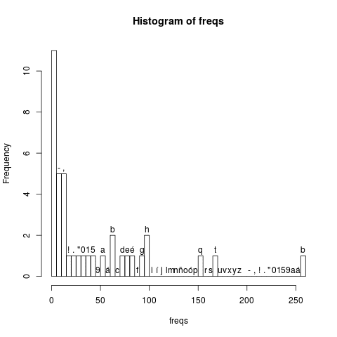
Here is a example on a text that is captured from the Oracle - History of Java site. The code below defines a large string. The string is then parsed into its characters. After calculating the frequencies of each single character (including numbers, commas and dots) a histogram is saved in a file.






# Defining string 
s <- "Since 1995, Java has changed our world and our expectations. Today, with technology such a part of our daily lives, we take it for granted that we can be connected and access applications and content anywhere, anytime. Because of Java, we expect digital devices to be smarter, more functional, and way more entertaining. In the early 90s, extending the power of network computing to the activities of everyday life was a radical vision. In 1991, a small group of Sun engineers called the \"Green Team\" believed that the next wave in computing was the union of digital consumer devices and computers. Led by James Gosling, the team worked around the clock and created the programming language that would revolutionize our world – Java. The Green Team demonstrated their new language with an interactive, handheld home-entertainment controller that was originally targeted at the digital cable television industry. Unfortunately, the concept was much too advanced for the them at the time. But it was just right for the Internet, which was just starting to take off. In 1995, the team announced that the Netscape Navigator Internet browser would incorporate Java technology.Today, Java not only permeates the Internet, but also is the invisible force behind many of the applications and devices that power our day-to-day lives. From mobile phones to handheld devices, games and navigation systems to e-business solutions, Java is everywhere!"

# First converting to lower case
# then splitting by characters.
# strsplit return a list, we are unlisting to a vector.
chars <- unlist(strsplit(tolower(s), ""))

# Generating frequency table
freqs <- table(chars)

# Generating plot into a file
png("Graph.png")
hist(freqs,include.lowest=TRUE, breaks=46,freq=TRUE,labels=rownames(freqs))
dev.off()



The generated output is

We translate the text used in our example to Spanish using Google Translate site. The code is shown below:

# Defining string 
s <- "Desde 1995, Java ha cambiado nuestro mundo y nuestras expectativas. Hoy en día, con la tecnología de una parte de nuestra vida cotidia    na tal, damos por sentado que se puede conectar y acceder a las aplicaciones y contenido en cualquier lugar ya cualquier hora. Debido a Java    , esperamos que los dispositivos digitales para ser más inteligente, más funcional, y de manera más entretenida. A principios de los años 90    , que se extiende el poder de la computación en red para las actividades de la vida cotidiana era una visión radical. En 1991, un pequeño gr    upo de ingenieros de Sun llamado \"Green Team\" cree que la próxima ola de la informática fue la unión de los dispositivos digitales de cons    umo y ordenadores. Dirigido por James Gosling, el equipo trabajó durante todo el día y creó el lenguaje de programación que revolucionaría e    l mundo - Java. El Equipo Verde demostró su nuevo idioma con una mano controlador interactivo, el entretenimiento en casa que fue dirigido o    riginalmente a la industria de la televisión digital por cable. Por desgracia, el concepto fue demasiado avanzado para el ellos en el moment    o. Pero fue justo para Internet, que estaba empezando a despegar. En 1995, el equipo anunció que el navegador de Internet Netscape Navigator     incorporaría Java technology.Today, Java no sólo impregna el Internet, pero también es la fuerza invisible detrás de muchas de las aplicaci    ones y dispositivos que alimentan nuestra vida del día a día. Desde teléfonos móviles para dispositivos de mano, juegos y sistemas de navega    ción para e-business soluciones, Java está en todas partes!"

# First converting to lower case
# then splitting by characters.
# strsplit return a list, we are unlisting to a vector.
chars <- unlist(strsplit(tolower(s), ""))

# Generating frequency table
freqs <- table(chars)

# Generating plot into a file
png("Graph.png")
hist(freqs,include.lowest=TRUE, breaks=46,freq=TRUE,labels=rownames(freqs))
dev.off()

The generated plot for the Spanish translation is:

Note that some characters such as space, dots and commas can be replaced from the string s using a code similar to this:

news <- gsub(pattern=c(" "), "", x=s)

The code above removes all spaces from the string s and a new string variable news holds the modified string. Original variable remains same. 

Have a nice read!

Environments in R

An environment is a special term in R, but its concept is used in many interpreters of programming languages. The term of variable scope is directly related with environments. An environment in R encapsulates a couple of variables or objects which itself is encapsulated by a special environment called global environment.

After setting a variable to a value out of any function and class, the default holder of this variable is the global environment.

Suppose we set t to 10 by

t <- 10

and this is the same as writing


assign(x="t", value=12, envir=.GlobalEnv)


and the value of t is now 12:


> t <- 10
> assign(x="t", value=12, envir=.GlobalEnv)
> t
[1] 12

Instead of using the global environment, we can create new environments and attach them to parent environments. Suppose we create a new environment as below:


> my.env <- new.env()
> assign(x="t", value="20", envir=my.env)
> t
[1] 12

Value of t is still 12 because we create an other t variable which is encapsulated by the environment my.env.


Variables in environments are accessable using the assign and the get functions.


> get(x="t", envir=my.env)
[1] "20"
> get(x="t", envir=.GlobalEnv)
[1] 12

As we can see, values of the variables with same name are different, because they are encapsulated by separate environments.

exists() function returns TRUE if an object exists in an environment else returns FALSE. Examining existence of an object is crucial in some cases. 

> exists(x="t", envir=.GlobalEnv)

[1] TRUE

> exists(x="t", envir=my.env)

[1] TRUE

> exists(x="a", envir=my.env)

[1] FALSE

 is.environment() function returns TRUE if an object is an environment else returns FALSE. 

> is.environment(.GlobalEnv)

[1] TRUE

> is.environment(my.env)

[1] TRUE

> is.environment(t)

[1] FALSE

Finally, environments are simply lists and a list can be converted to an environment easly. 

> my.list <- list (a=3, b=7)
> my.env <- as.environment(my.list)
> get("a", envir=my.env)
[1] 3
> get("b", envir=my.env)
[1] 7

The inverse process is converting an environment to a list: 

> as.list(.GlobalEnv)

$t

[1] 12

$my.env

$my.list

$my.list$a

[1] 3

$my.list$b

[1] 7

Happy R days :)

Fast and robust estimation of regression coefficients with R

Outliers are aberrant observations that do not fit the remaining of the data, well. In regression analysis, outliers should not be distant from the remaining part, that is, if an observation is distant from the unknown regression object (a line in two dimensional space, a plane in three dimensional space, a hyper-plane in more dimensional space, etc.) it is said to be an outlier. If the observation is distant from the regression object by its independent variables, it is called bad leverage. If an observation is distant by its dependent variables, it is said to be regression outlier. If it is distant by both of the dimensions, it can be a good leverage, which generally reduces the standard errors of estimates. Bad leverages may result a big difference in estimated coefficients and they are accepted as more dangerous in the statistics literature.

Since an outlier may change the partial coefficients of regression, examining the residuals of a non-robust estimator results wrong conclusions. An outlier may change one or more regression coefficients and hide itself with a relatively small residual. This effect is called masking. This change in coefficients can get a clean observation distant from the regression object with higher residual. This effect is called swamping. A successful robust estimator should minimize these two effects to estimate regression coefficients in more precision.

The medmad function in R package galts can be used for robust estimation of regression coefficients. This package is hosted in the CRAN servers and can be installed in R terminal by typing


install.packages("galts")


Once the package is installed, its content can be used by typing


require("galts")


and the functions and help files can be ready to use after typing an enter key.  Here is a complete example of generating a regression data, contaminating some observations and estimating the robust regression coefficients:

The output is

(Intercept)          x1          x2 
4.979828          4.993914    4.985901 

and the medmad function returns in 0.25 seconds in an Intel i5 computer with 8 GBs ram installed.

in which the parameters are near to 5 as the data is generated before. The details of this algorithm can be found in the paper

Satman, Mehmet Hakan. "A New Algorithm for Detecting Outliers in Linear Regression." International Journal of Statistics and Probability 2.3 (2013): p101.

which is avaliable at site

http://www.ccsenet.org/journal/index.php/ijsp/article/view/28207

and

http://www.ccsenet.org/journal/index.php/ijsp/article/download/28207/17282


Have a nice detect!

Word Cloud Generation Using Google Webmaster Tools Data and R

In this blog entry, we generate a word cloud graphics of our blog, stdioe, using the keyword data in Google Webmaster Tools. In webmaster tools site, when you follow

Google Index -> Content keyword

you get the keywords with their frequencies. This data set can be saved in csv format using the button "Download this table".

The csv data for our blog was like this:

One can load this file and generate a word cloud graphics using R, and our code is shown below:

require("wordcloud")
 
mydata <- read.csv("data.csv", sep=";", header=TRUE)
 
png("stdioe_cloud.png",width=1024, height=768)
wordcloud(words=mydata$Keyword, freq=mydata$Occurrences,scale=c(10,1))
dev.off()

The generated output is:

Here is the stdioe's search query keywords cloud:

Matrix Inversion with RCaller 2.2

Here is the example of passing a double[][] matrix from Java to R, making R calculate the inverse of this matrix and handling the result in Java. Note that code is current for 2.2 version of RCaller.

RCaller caller = new RCaller(); 
Globals.detect_current_rscript(); 
caller.setRscriptExecutable(Globals.Rscript_current); 

RCode code = new RCode(); 

double[][] matrix = new double[][]{{6, 4}, {9, 8}};

code.addDoubleMatrix("x", matrix); 
code.addRCode("s<-solve font="" x="">); 

caller.setRCode(code); 

caller.runAndReturnResult("s"); 

double[][] inverse = caller.getParser().getAsDoubleMatrix("s", 

                                       matrix.length, matrix[0].length); 

        
for (int i = 0; i < inverse.length; i++) {
    for (int j = 0; j < inverse[0].length; j++) {

        System.out.print( inverse[i][j] + " ");

    } 

    System.out.println();
} 
 

A gWidgets Example - Using windows, groups, labels, text and password boxes, buttons and events in R

A gWidget Example - Using windows, groups, labels, text and password boxes, buttons and events in R

jbytecode

August 20, 2013

In this entry, a short example for using gWidgets is given. gWidgets is a package for creating GUI’s in R.

Our example shows a GUI window with width = 400 and height = 400. Window is created by gwindow function. Components are located by rows. Rows are handled by ggroup function. ggroup must take a container as a parameter. In this logic, lbl_username and txt_username are childs of row1 which is child of gwindow.

Any text field can act as a password field by using visible¡- function.

visible(txt_password) <- FALSE

So, the object txt_password is now hiding characters by * characters. Finally, the method addHandlerClicked links an object to a function for click event. In our example, btn_login is linked to do_login function. When btn_login clicked, a message is written. The source code of the complete example is given below.

 
1# Loading required packages 
2require("gWidgets") 
3require("gWidgetstcltk") 
4 
5# main window 
6main <- gwindow(title="Login␣Window", 
7                width=400, 
8                height=400) 
9 
10# a row and components 
11row1 <- ggroup(container=main) 
12lbl_username <- glabel(container=row1, text="Username:␣") 
13txt_username <- gedit(container=row1) 
14 
15 
16# a row and components 
17row2 <- ggroup(container=main) 
18lbl_password <- glabel(container=row2, text="Password:␣") 
19txt_password <- gedit(container=row2) 
20 
21# any text in txt_password will be show with * character 
22visible(txt_password) <- FALSE 
23 
24# a row for button 
25row3 <- ggroup(container=main) 
26btn_login <- gbutton(container=row3, 
27                        text="Login") 
28btn_register <- gbutton(container=row3, 
29                        text="Register") 
30 
31 
32# Event handler for login button 
33do_login <- function(obj){ 
34        cat("Login␣with␣",svalue(txt_username),"\n") 
35} 
36 
37# Event handler for register button 
38do_register <- function(obj){ 
39        cat("Register␣with␣", svalue(txt_username),"\n") 
40} 
41 
42 
43# Registering Events 
44addHandlerClicked ( btn_login, do_login) 
45addHandlerClicked ( btn_register, do_register)

Generating LaTeX Tables in R

Generating LATEXTables in R

jbytecode

August 18, 2013

Many R users prepare reports, documents or research papers using LATEXtype-setting system. Since typing tabular data structures in LATEXby hand consumes too much construction time, some packages were developed for automatic creation or conversion of R datasets. In this short entry, we show the usage and output of xtable function in xtable package. First install the package if it is not already installed:

> install.packages(”xtable”)

After installation, the package is loaded once in the current session:

> require(”xtable”)

Now, suppose that we have a data frame and we want to export it as a LATEXtable. Let’s create a random dataset with three variables, x,y and z.

> x<-round(runif(10,0,100)) 
> y<-round(runif(10,0,100)) 
> z<-round(runif(10,0,100)) 
> data <- as.data.frame ( cbind(x,y,z) ) 
> data 
    x   y  z 
1  26  86 44 
2  81  13 22 
3  39  27 57 
4  32  57 56 
5  50  15 31 
6  34 100 98 
7  54  46 24 
8  42  55 42 
9  62  91 77 
10  5  73 25

Calling the function xtable simply on the data that we have just created produces some output:

> xtable(data)

% latex table generated in R 2.15.3 by xtable 1.7-1 package  
% Sun Aug 18 23:40:23 2013  
\begin{table}[ht]  
\centering  
\begin{tabular}{rrrr}  
  \hline  
 & x & y & z \\  
  \hline  
1 & 26.00 & 86.00 & 44.00 \\  
  2 & 81.00 & 13.00 & 22.00 \\  
  3 & 39.00 & 27.00 & 57.00 \\  
  4 & 32.00 & 57.00 & 56.00 \\  
  5 & 50.00 & 15.00 & 31.00 \\  
  6 & 34.00 & 100.00 & 98.00 \\  
  7 & 54.00 & 46.00 & 24.00 \\  
  8 & 42.00 & 55.00 & 42.00 \\  
  9 & 62.00 & 91.00 & 77.00 \\  
  10 & 5.00 & 73.00 & 25.00 \\  
   \hline  
\end{tabular}  
\end{table}

The generated output can easly be integrated with an LATEXfile. This table is shown as

---

	x	y	z
1	26.00	86.00	44.00
2	81.00	13.00	22.00
3	39.00	27.00	57.00
4	32.00	57.00	56.00
5	50.00	15.00	31.00
6	34.00	100.00	98.00
7	54.00	46.00	24.00
8	42.00	55.00	42.00
9	62.00	91.00	77.00
10	5.00	73.00	25.00

---

This is an example of xtable function call with default parameters. In the next example, we put a caption.

> xtable(data,caption=”Our random dataset”)

---

	x	y	z
1	26.00	86.00	44.00
2	81.00	13.00	22.00
3	39.00	27.00	57.00
4	32.00	57.00	56.00
5	50.00	15.00	31.00
6	34.00	100.00	98.00
7	54.00	46.00	24.00
8	42.00	55.00	42.00
9	62.00	91.00	77.00
10	5.00	73.00	25.00

Table 1: Our random dataset

---

Let’s put a label on it:

> xtable(data,caption=”Our random dataset”, 
                          label=”This is a label”)

---

	x	y	z
1	26.00	86.00	44.00
2	81.00	13.00	22.00
3	39.00	27.00	57.00
4	32.00	57.00	56.00
5	50.00	15.00	31.00
6	34.00	100.00	98.00
7	54.00	46.00	24.00
8	42.00	55.00	42.00
9	62.00	91.00	77.00
10	5.00	73.00	25.00

Table 2: Our random dataset

---

And this function call shows the numbers with three fractional digits.

> xtable(data,caption=”Our random dataset”, 
                label=”This is a label”, 
                digits=3)

---

	x	y	z
1	26.000	86.000	44.000
2	81.000	13.000	22.000
3	39.000	27.000	57.000
4	32.000	57.000	56.000
5	50.000	15.000	31.000
6	34.000	100.000	98.000
7	54.000	46.000	24.000
8	42.000	55.000	42.000
9	62.000	91.000	77.000
10	5.000	73.000	25.000

Table 3: Our random dataset

---

Sorting Multi-Column Datasets in R

Sorting Multi-Column Datasets in R

August 18, 2013

In this entry, we present the most straightforward way to sort multi-column datasets

Suppose that we have a vector in three dimensional space. This vector can be defined as

a <- c(3,1,2)

in R. The built-in function sort sorts a given vector in ascending order by default. An ordered version of vector a is calculated as shown below:

sorted_a <- sort(a)

The result is

[1] 1 2 3

For reverse ordering, the value of decreasing parameter must be set to TRUE.

> sort(a,decreasing=TRUE) 
[1] 3 2 1

Another related function order returns indices of sorted elements.

> a <- c(3,1,2) 
> order (a) 
[1] 2 3 1

In the example above, it is shown that if the vector a is ordered in ascending order, second element of a will be placed at index 1. It is easy to show that, result of the function order can be used to sort data.

> a <- c(3,1,2) 
> o <- order (a) 
> a[o] 
[1] 1 2 3

Suppose that we need to sort a matrix by a desired row. The solution is easy. Get the indices of sorted desired column and use the same method as in example given above.

> x <- round(runif(5, 0, 100)) 
> y <- round(runif(5, 0, 100)) 
> z <- round(runif(5, 0, 100)) 
> data <- cbind(x,y,z) 
> data 
      x  y  z 
[1,] 48 35 75 
[2,] 40 21 43 
[3,] 58 69  1 
[4,] 49 38  2 
[5,] 43 66 46

Now, get the indices of sorted z:

> o <- order(z) 
> data[o,] 
      x  y  z 
[1,] 58 69  1 
[2,] 49 38  2 
[3,] 40 21 43 
[4,] 43 66 46 
[5,] 48 35 75

Finally, we sorted the dataset data by the column vector z.